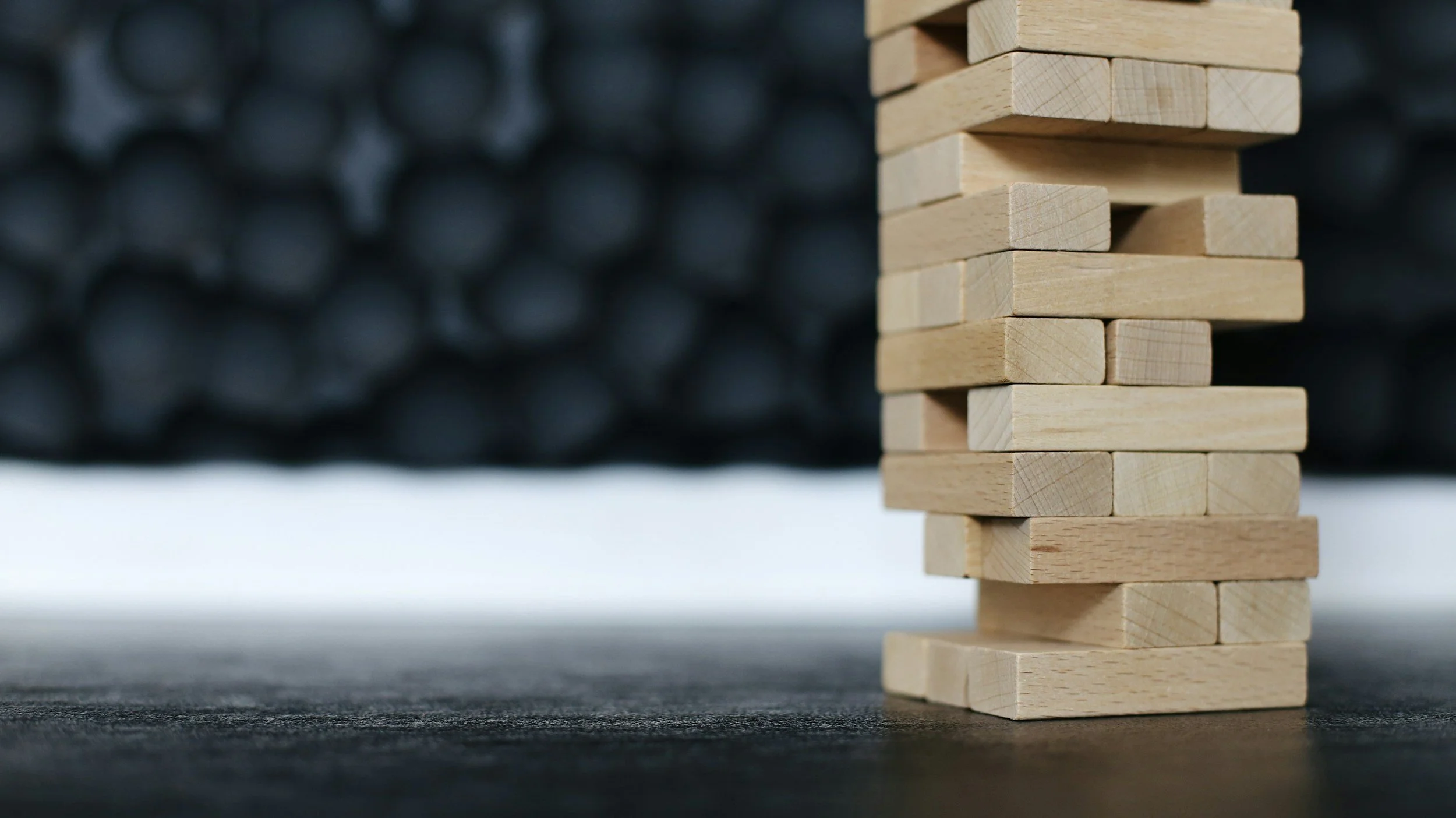
5 DOF Arm Jenga Block Stacking
The goal was to balance speed, accuracy, and control
-
Forward kinematics (FK) is the connection between the joint angles and the end effector location. While not being critical for the feed forward control of a robotic arm, FK will be helpful for gathering key waypoints in the cartesian space.
-
Inverse kinematics (IK) are the, well inverse of the forward kinematics. They represent the relationship between the end effector location and the joint angles. IK is what will be used to actually control the location of the end effector.
-
Unfortunately, joints have backlash and friction, not to mention that variable torque is required to drive the joints depending on robot state due to gravity. Errors in the joint position can be accounted for with a closed loop PID control scheme on each joint.
-
While the PID control can compensate for gravity to some extent, it was far more effective to calculate the torque applied to each joint as a result of gravity and account for it directloy.
-
Simply picking a single rotational speed for every waypoint-to-waypoint motion would either result in overshoot or slower than necessary travel. Implementing trapezoidal velocity profile allows for the best of both worlds
-
Ultimately a lot of time went in to selecting the ideal waypoints to avoid block collisions during placement.
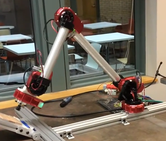
The arm
The arm is constructed as a 5 degree of freedom rotational (RRRRR) arm. This means that there are 5 actuators in series (but on different axes) that allow the robot to move. The end effector is an actively controlled suction cup that allows for blocks to be picked up from the feeder.
Forward Kinematics
The forward kinematics are relatively easy to solve for. While not directly used in the placement script, this is a useful tool to have. FK can be found using basic trigonometry and adding the rotational and translational contribution of every joint given joint angles.
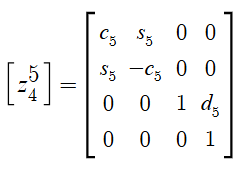
Denavit Hartenberg parameters are an algorithmic way of arriving at the FK equation for a given robotic system. By defining coordinate frames at every joint such that the axis of rotation falls on the Z axis and the link to the next joint falls on the X axis, we are able to define the matrix to the right as the general transformation between joint i and joint i+1.
The thetas represent the joint angle, the the d represents the distance traveled along the resulting direction. It is essentially a squerical cordinate, although we are stuck at a given z height because a rotational joint sweeps a plane.
By stacking multiple of these transformation matrices together as follows, we can get the transformation matrix between the origin and end effector:

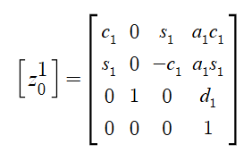
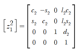
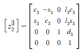
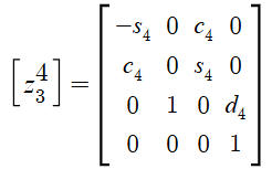
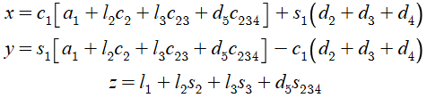
Resulting in these forward kinematics equations:
Inverse Kinematics
Inverse Kinematics are a little more difficult to solve for. However, working joint by joint we can simplify to a more familiar arm (RR) and go from there.
First we can easily solve for θ₁. We know that the end effector must be at x,y,z. We can simply take the atan of the x and y positions to get θ₁ with some additional caveats. Firstly, we need to use atan2. This allows for a 360 degree mapping and dodges the tan(θ)=tan(θ+180) issue. Second, we need to account for the joint offsets d₁, d₂, d₃ which affect the angle θ₁:

We can also get θ₅ pretty easily because it only depends on θ₁ and the end effector orientation matrix (which is a given for inverse kinematics):

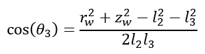
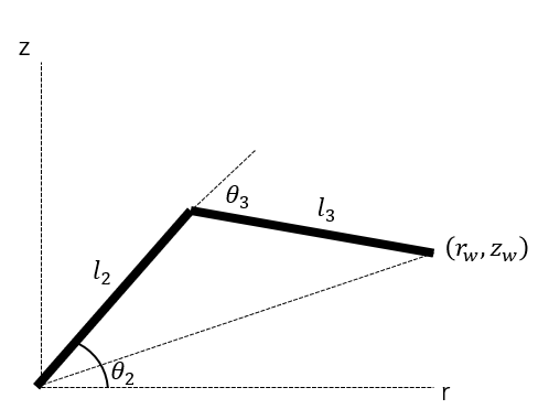
Now we simplify. First we work back from the end effector to the wrist (location of joint 4). This allows us to view joints 2 and 3 as part of the aforementioned planar RR arm.

This simplification allows us to use basic trig to arrive at θ₃:

And θ₂:

Lastly, θ₂, θ₃, and θ₄, all contribute to end effector pitch which allows us to solve for θ₄

Now we can input our intended end effector coordinates and get back out the joint angles needed to reach those coordinates!
Joint Control
Control could be a whole other topic, so I’ll keep it brief. You can read more about PID control schemes from my one cookie oven project
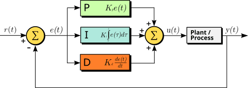
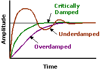
Just because we tell a joint to go to a specific orientation does not mean that it will go exactly there. It may overshoot, undershoot, oscillate between the two etc. We can tune this by changing the proportional, integral, and derivative terms in each joints feedback loops.
Proportional looks at the current distance between the position and commanded position. This is the main driver of joint command. This allows us to move towards the goal.
Integral looks at the area under the proportional curve. In other words, the longer we have positional error, the higher the integral term gets. This allows us to remove steady state errors.
The derivative term responds to the speed of the joint. Often this is a negative term that causes the joint to slow down. It is normally present to decrease overshoot at the cost of movement speed.
In this case, we tuned each one of these by hand (although there are algorithms to help with this).
It was crucial to not overshoot by too much as that could break the robot or nock over the tower.
It was also important to be accurate with our final location to ensure good picks and places.
Finally, we pushed for as little derivative control as possible without hurting the previous two points to make our cycles run as quickly as possible.
The green curve to the right was the goal for each joint, but again, this depended on the robot state, so we optimized around the rough state when placing a block, and that was good enough for the rest of the robot range - almost
Gravity Compensation
Again, I wont go into too much detail here. Just enough to explain, well, the gravity of the situation
Imagine the arm is perfectly upright. There are no torques as a result of gravity on any of the joints. In fact, joint 1 is never affected by gravity (the joint axis runs parallel with gravity) and joint 5 would only have a gravity applied torque if it grabbed another object off center. Joints 2, 3, and 4 however can be directly affected by gravity. Now imagine that the arm is perfectly horizontal. Every member, joint, and carried object will cause a torque on the joints that precede it. We can solve for this using physics and sum the moment contributions from each component about a given joint. OR… We can use the Jacobean!
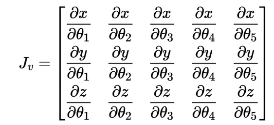
The Jacobean is defined like this:
It describes the contribution to the motion of the end effector of each joint for each cardinal direction. We can also come up with similar Jacobeans that describe the same behavior for each other mass. In other words, how much does each joint contribute to the motion of each other actuator or member in a given direction. Luckily, most of these come for free due to our having calculated the forward kinematics! Because we are only focused on the torque due to gravity, we only need the last row of the Jacobeans. Summing these as follows, we can get the total torque due to gravity on each joint that we need to compensate for.
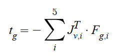
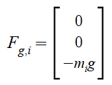
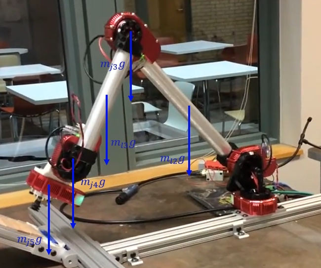
This will result in a torque vector that describes the additional torque needed to maintain the current robot state, without relying on each joint’s PID loop. This causes smoother and more accurate positioning.
Trajectory Control
The final lever we have to affect the accuracy and speed of the arm is to simply control the speed at which we ask the joints to travel. The obvious answer would be to set the joints to move at maximum speed until they reach their destination angles defined by IK. However, this kind of scheme causes lots of violent motion and jerkiness. The PID control should help with this, but we only care to be accurate at the beginning and end of a given travel path and can be faster and more inaccurate in the middle of the path. As a result, it makes sense to ramp up the speed from 0 to full speed linearly over some initial duration, travel at max speed, and then ramp down speed as the destination is approached. Implementing this was very simple, as we could provide a duration during which the robot would move from one waypoint to another. The PID values can then be optimized around slower speeds.
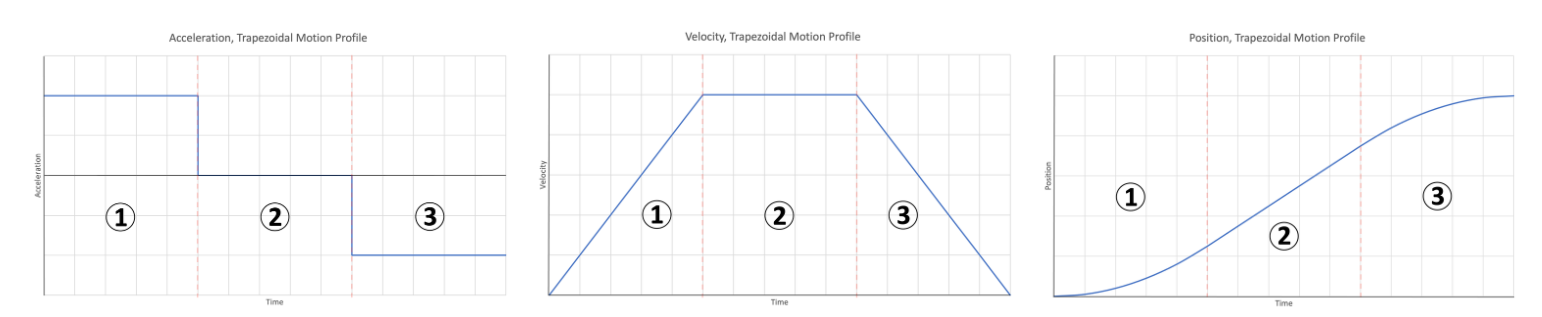
Image from Mechatronics Studio
Waypoint Tweaking
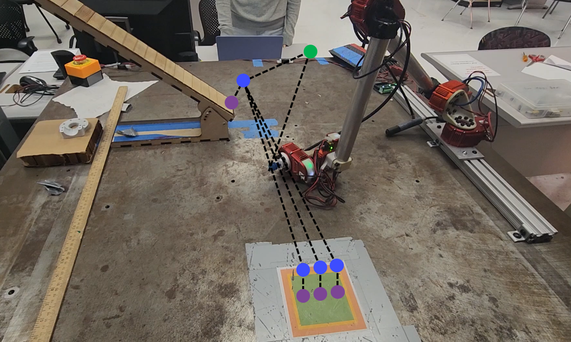
There are a few key waypoints that the robot needed to reach. Specifically, the block feeder, and the location rotation of each of the blocks in the tower. These could be optimized experimentally to find waypoints that most often resulted in successful pick-ups or placements. Ultimately, due to the flexibility of the end effector and the tight proximity of the placed blocks, it became clear that adding additional waypoints right above the block landing zone was necessary. Essentially these additional waypoints forced the arm to move perfectly vertically up from the block after placement to prevent dragging until the end effector was no longer in contact and then proceed to pick up the next block.
The image to the right shows the rough waypoint pathway for the first layer of blocks. The green way point was added to avoid collisions for most starting conditions, then the robot would make its way between the purple points, always stopping at the appropriate blue points on the way. The other layers were just the same thing with Z offsets and the appropriate 90-degree rotations on alternate layers.
Stackin Blocks!
(before final waypoint tweaking)